Weather model

Background

Weather affects both supply and demand for electricity. It determines the output of solar and wind power plants and drives electricity consumption. Because supply and demand set prices, weather has a strong influence on electricity market prices.

We have developed a unified, global weather model that creates realistic future weather data. Given a location and a time range, the Tensor weather model creates weather data up to the end of 2095. A simulation must start before 2040.

The weather model takes historical weather data and projects it into the future, so each point in time in the simulated future corresponds to a specific point in time in the past. For example, future weather for April 1st, 2030 is the weather recorded on April 1st, 2014.

For the same reason, the weather model cannot provide meaningful short-term forecasts. It is neither a physical simulation of the planetary weather system, which would require a supercomputer, nor a deep learning forecasting model such as Google GraphCast.

As explained in the introduction, the Tensor Cloud simulation engine uses future weather data as an input for:

• Solar and battery storage asset simulation
• Creation of electricity price forward curves
• Curtailment simulation

Development goals

Our primary goal for the Tensor weather model was bankability. We focused on three levers that we consider prerequisites for a bankable renewable energy or storage project: explainability, statistical accuracy, and internal consistency.

Explainability

You can trace every year of future weather to a specific year in the past by following the model's calculation logic below. We chose not to generate weather synthetically (for example, with a TMY approach) so that you can trace the data lineage of every simulation result.

Statistical accuracy

Over a long time horizon, this approach is also more accurate than alternatives that repeat the same year. A continuous time series that replays decades of past weather actuals keeps the full randomness of historical weather, so the digital twins of your assets are exposed to spikes of extreme heat or rain as they would be in reality.

The trade-off shows up at shorter timescales. Over years the approach is more accurate, but it can be a problem for an asset manager who compares real asset performance with simulation results month by month.

A TMY (typical meteorological year) approach gives results that are more homogeneous at monthly resolution. Talk to us if you are interested in using TMY weather in addition to the Tensor weather model.

Internal consistency

To simulate assets in the future, we need weather data for any location in Japan, and the data for different locations must be coherent: assets in the same zone should experience similar weather, and all assets should experience the same prices with the correct correlation to their weather. To achieve this, we take weather data from the past and re-index it to the future.

The simulation uses the weather at the asset location to estimate solar generation, and the weather at specific reference points as inputs to the price generation model. Solar generation at each plant is therefore correlated with the prices that the plant receives.

Example

On a sunny day in Kyushu, a plant produces a lot of electricity, but so do many other plants, and prices drop to zero. Without this correlation, the simulation could not show that the plant earns no revenue while it is at peak output.

Climate change

The Tensor weather model does not currently consider the impact of climate change, because it repeats weather from the past. Our research team is looking into ways to incorporate long-term IPCC scenarios with rising temperatures and more extreme weather events.

Tensor Cloud is not a climate risk management platform, and long-term climate predictions are highly uncertain, so we follow the common practice in the renewable energy industry of leaving climate change out of asset simulation models.

Calculation logic

Boundary between actual and historical data

The split between "past" (actual recorded weather) and "future" (mapped historical weather) is not fixed. It is set 5 days before the simulation run date (midnight, Japan time), so that only recorded weather that is already available is used. Everything before this boundary uses actual recorded weather; everything after it uses historical weather mapped with the formula below.

Time periods in the past

For time periods in the past (for assets with a COD in the past, up to the present), we use actual weather data from the asset's location.

Time periods in the future

For future dates, we map past weather actuals to those dates: we take past weather for the same period of the year and re-index it to the future. For each year $Y$ in the past, we assign a new year $Y'$ defined as:

$$Y' = Y + (252 - \left \lfloor \frac{Y}{8} \right \rfloor) \cdot 16$$

This produces meaningful dates for any year until 2095, and the nearer future is simulated with weather from the more recent past. From 2096 onward, the mapping would point to years before 1940, where no reanalysis data exists.

Future years are mapped in 8-year blocks that follow the calendar, not the asset's COD: each block ends on January 1st of a year divisible by 8 (2032, 2040, and so on). Consecutive blocks overlap by one day, and the first reading available at each hour is used.

info

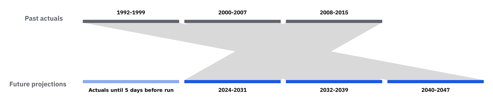
With this mapping, future periods correspond to the following periods in the past:

period 2024-2031 -> mapped to 2008-2015
period 2032-2039 -> mapped to 2000-2007
period 2040-2047 -> mapped to 1992-1999

Future periods are never mapped to weather from 2016 onward. Our price model is trained on recent years, so this keeps the weather it was trained on out of the inputs it receives for future prices. Recent weather is still used for actual past periods and for the exceedance scenarios.

Data sources

Our historical weather data comes from several datasets, accessed through the Open-Meteo historical weather archive. For each location, we combine these datasets to get the most accurate historical weather conditions.

ERA5-Land supplies air temperature only; irradiance and wind speed come from ERA5 and ECMWF IFS. Because future periods are mapped to years before 2016, all future irradiance comes from ERA5 at 0.25° resolution. ECMWF IFS data, available from 2017, affects only actual past periods.

If an hour of weather is missing, it is bridged from the readings on either side. If a longer gap remains, the simulation stops with an error instead of producing a result with missing generation.

Data set	Spatial resolution	Temporal resolution	Data availability	Update frequency
ECMWF IFS	9 km	1 hour	2017 to present	Daily with 2 days delay
ERA5	0.25° (~25 km)	1 hour	1940 to present	Daily with 5 days delay
ERA5-Land	0.1° (~11 km)	1 hour	1950 to present	Daily with 5 days delay

Re-running simulations

Why results differ when re-running a simulation

When you re-run a simulation on a different date, the boundary between actual and historical weather shifts. For example, a simulation run on March 31st treats March 26th onward as "future", while the same simulation run on April 10th treats April 5th onward as "future". For the roughly 10 days between these two boundaries:

• The March 31st run used weather from 16 years ago for that period
• The April 10th run used actual 2026 recorded weather, which had become available by then

Irradiance and temperature for that period therefore differ slightly, and so does simulated generation.

Why differences can extend beyond the first year

The weather itself changes only between the two boundaries. The 8-year blocks are fixed to the calendar, so the run date moves where actual weather ends but not where any block ends, and the weather after the later boundary is the same in both runs.

Results in later years can still differ slightly because of curtailment. Curtailment events for every fiscal year are drawn in sequence from one random sequence fixed by the asset's location. When the generation in the changed period alters the number of events drawn in that year, the events drawn for the following years can change too.

Exceedance scenarios can also change when a simulation is re-run in a new calendar year, as the interannual variability is measured over the last 20 full years.

Further reading

• Tensor Cloud simulations: Use weather-based generation estimates in project return analysis.
• Research on Japan's solar growth: See the broader solar deployment context for generation modeling.